Particle analysis
This example demonstrates how to analyze the shape of objects (‘particles’) in a binary image.
First, the example generates artificial particles using the sphere and box commands.
def generate_particles(sphere_count=1000, box_count=1000):
        """
        analyze_particles demo uses this to generate an image containing some random regions.
        """

        import random

        img = pi.newimage(ImageDataType.UINT8, 500, 500, 500)

        # Generate some spheres
        for i in range(0, sphere_count):
                pos = [random.randint(0, 500), random.randint(0, 500), random.randint(0, 500)]
                r = random.randint(1, 20)
                pi.sphere(img, pos, r, 255)

        # Generate some boxes
        for i in range(0, box_count):
                pos = [random.randint(0, 500), random.randint(0, 500), random.randint(0, 500)]
                size = [random.randint(1, 20), random.randint(1, 20), random.randint(1, 20)]
                pi.box(img, pos, size, 255)

        pi.writeraw(img, output_file('particles'))
Next, the available analyzers are queried using command listanalyzers. The command lists all available analyzers and columns they produce to the output. At the time of writing the analyzers are
coordinates
Shows (zero-based) coordinates of a pixel that is guaranteed to be inside the particle. Output column names are ‘X’, ‘Y’, and ‘Z’.
isonedge
Tests whether the particle touches image edge. If it does, returns 1 in a column ‘Is on edge’; if it doesn’t, returns zero.
volume
Shows total volume of the particle in pixels. Outputs one column with name ‘Volume’.
pca
Calculates orientation of the particle using principal component analysis. Outputs:
Centroid of the particle in columns ‘CX’, ‘CY’, and ‘CZ’.
Meridional eccentricity in column ‘e (meridional)’.
Standard deviations of the projections of the particle points to the principal axes in columns ‘l1’, ‘l2’, and ‘l3’.
Orientations of the three principal axes of the particle, in spherical coordinates, in columns ‘phiN’ and ‘thetaN’, where N is in 1…3, phiN is the azimuthal angle and thetaN is the polar angle.
Maximum distance from the centroid to the edge of the particle in colum ‘rmax’.
Maximum diameter of the projection of the particle on each principal component in columns ‘d1’, ‘d2’, and ‘d3’.
Scaling factor for a bounding ellipsoid in column ‘bounding scale’. An ellipsoid that bounds the particle and whose semi-axes correspond to the principal components has semi-axis lengths \(b lN\), where \(b\) is the bounding scale and \(lN\) are the lengths of the principal axes.
surfacearea
Shows surface area of particles determined with the Marching Cubes method. Outputs one column ‘Surface area’.
bounds
Calculates axis-aligned bounding box of the particle. Returns minimum and maximum coordinates of particle points in all coordinate dimensions. Outputs columns ‘minX’ and ‘maxX’ for each dimension, where X is either x, y, or z.
boundingsphere
Shows position and radius of the smallest possible sphere that contains all the points in the particle. Outputs columns ‘bounding sphere X’, ‘bounding sphere Y’, ‘bounding sphere Z’, and ‘bounding sphere radius’. Uses the MiniBall algorithm from Welzl, E. - Smallest enclosing disks (balls and ellipsoids).
The actual particle analysis is performed with analyzeparticles command. It needs as input the binary image, image for results, and a string that contains the names of the desired analyzers.
The output image contains one row for each particle in the image. The meanings of columns can be found using command
headers. Its output in this case is
Volume [pixel], X [pixel], Y [pixel], Z [pixel], minx, maxx, miny, maxy, minz, maxz, bounding sphere X [pixel], bounding sphere Y [pixel], bounding sphere Z [pixel], bounding sphere radius [pixel], Is on edge [0/1].
Finally, the results are converted to NumPy format and the volume distribution of the particles is plotted.
def analyze_particles():
        """
        Demonstrates particle (i.e, region or blob) analysis, and some drawing commands.
        """

        # Generate particle image
        generate_particles()

        # Show analyzer names.
        # This does not do anything else than shows which analyzers are available.
        pi.listanalyzers()

        # Make a list of analyzers that we want to use
        analyzers = 'volume coordinates bounds boundingsphere isonedge'


        # Read generated data file
        img = pi.read(output_file('particles'))

        # Analyze particles
        result = pi.newimage(ImageDataType.FLOAT32)
        pi.analyzeparticles(img, result, analyzers)

        # Show titles of data columns
        print('Titles of columns in data table:')
        pi.headers(analyzers)

        # Get result data from the pi2 system
        pa = result.get_data()

        # Volume is in the first column (see output of 'headers' command)
        volume = pa[:, 0]

        # Plot volume histogram
        import matplotlib.pyplot as plt
        plt.hist(volume, density=True, bins=30)
        plt.xlabel('Volume [pixel]')
        plt.ylabel('Probability')
        plt.tight_layout()
        plt.show(block=False)
        plt.savefig(output_file('volume_distribution.png'))
Output:
coordinates
Shows (zero-based) coordinates of a pixel that is guaranteed to be inside the particle. Output column names are X, Y, and Z.

isonedge
Tests whether the particle touches image edge. If it does, returns 1.0 in a column 'isonedge'; if it doesn't, returns zero.

volume
Shows total volume of the particle in pixels. Outputs one column with name 'volume'.

bounds
Calculates axis-aligned bounding box of the particle. Returns minimum and maximum coordinates of particle points in all coordinate dimensions. Outputs columns 'minX' and 'maxX' for each dimension, where X is either x, y, or z.

boundingsphere
Shows position and radius of the smallest possible sphere that contains all the points in the particle. Outputs columns 'bounding sphere X', 'bounding sphere Y', 'bounding sphere Z', and 'bounding sphere radius'.
Analyzing in 8 blocks.
Processing 464 particles on block edge boundaries...
Find edge points of particles...
Build forest...
Determine bounding boxes...
Divide boxes to a grid...
Determine overlaps...
Combine particles...
Analyze combined particles...
Titles of columns in data table:
Volume [pixel], X [pixel], Y [pixel], Z [pixel], minx, maxx, miny, maxy, minz, maxz, bounding sphere X [pixel], bounding sphere Y [pixel], bounding sphere Z [pixel], bounding sphere radius [pixel], Is on edge [0/1]
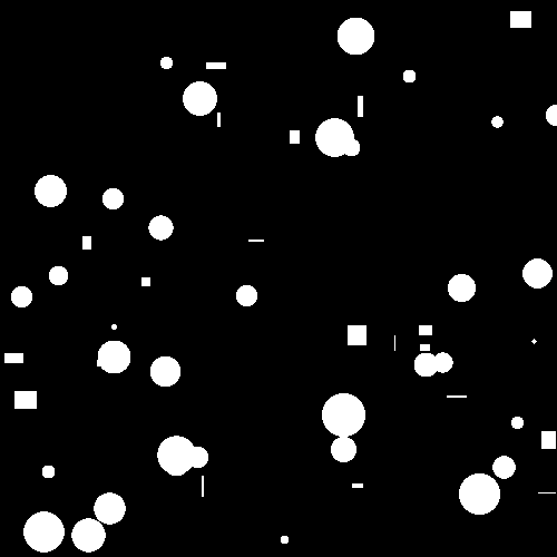
One slice of the input image. Background is black, particles are white.
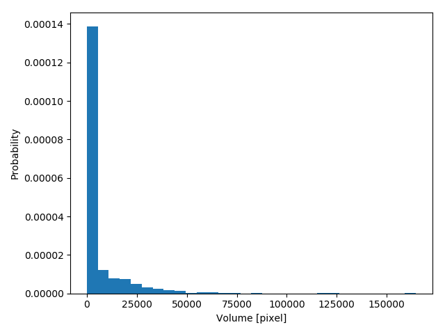
Distribution of particle volume.