Bivariate histogram

This example shows how to calculate the bivariate histogram of two images (of the same size). Here we calculate bivariate histogram of an image and its local thickness transform.

def bivariate_histogram():
        """
        Demonstrates determination of bivariate histogram.
        """

        # Read original
        img = pi.read(input_file())

        # Create a copy of the image and binarize it
        bin = pi.newlike(img)
        pi.copy(img, bin)
        pi.threshold(bin, 185)

        # Calculate thickness map.
        # Convert input image first to uint32 so that it can hold even large values.
        pi.convert(bin, ImageDataType.UINT32)
        tmap = pi.newlike(bin, ImageDataType.FLOAT32)
        pi.tmap(bin, tmap)

        # Calculate bivariate histogram of original and thickness map
        hist = pi.newimage(ImageDataType.FLOAT32)
        bins1 = pi.newimage(ImageDataType.FLOAT32)
        bins2 = pi.newimage(ImageDataType.FLOAT32)
        gray_max = 500   # Maximum gray value in the histogram bins
        thick_max = 30   # Maximum thickness in the histogram bins
        pi.hist2(img, 0, gray_max, 60, tmap, 0, thick_max, 15, hist, bins1, bins2) # 60 gray value bins, 15 thickness bins

        # Write output files to disk
        pi.writetif(img, output_file('original'))
        pi.writetif(tmap, output_file('thickness_map'))
        pi.writetif(hist, output_file('histogram'))
        pi.writetif(bins1, output_file('bins1'))
        pi.writetif(bins2, output_file('bins2'))

        # Get histogram data
        h = hist.get_data()

        # Make plot
        import matplotlib.pyplot as plt
        fig = plt.figure(figsize=(4.5, 6))

        # Note that here we plot the transpose of the histogram as that fits better into an image.
        # We also flip it upside down so that both x- and y-values increase in the usual directions.
        pltimg = plt.imshow(np.flipud(h.transpose()), vmin=0, vmax=1.5e4, extent=(0, thick_max, 0, gray_max), aspect=1/8)
        cbar = fig.colorbar(pltimg)
        plt.xlabel('Thickness [pix]')
        plt.ylabel('Gray value [pix]')
        cbar.set_label('Count', rotation=90)
        plt.tight_layout()
        plt.show(block=False)
        plt.savefig(output_file('bivariate_histogram.png'))

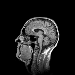
One slice of the input image.

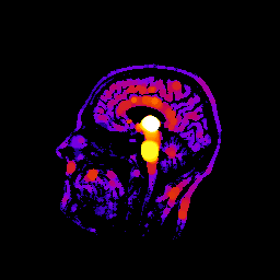
Local thickness map of the input. Brighter colors correspond to thicker regions.

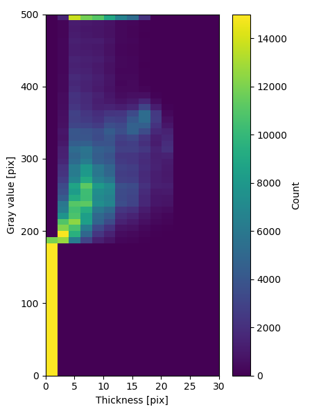
Bivariate histogram of local thickness and original gray value, showing that larger thicknesses tend to be found in brighter regions. The bright row at gray value \(500\) is caused by out-of-bounds values (gray value \(>500\)) included in the last bin.