Estimation of orientation using the structure tensor method
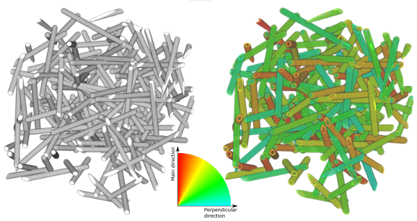
3D visualization of the generated input image (left panel), and similar visualization where the fibres have been colored according to the local orientation (right).
This example shows how to estimate orientation of cylindrical structures using the structure tensor method.
First, the example generates an image containing randomly oriented cylinders. Orientation of each cylinder is drawn from a von Mises-Fisher distribution, that allows specifying a main direction and spread of the orientations. The cylinders are drawn into a pi2 image. In the code below, the sampling procedure is skipped as it is somewhat lengthy and not directly related to pi2. The sampling code is shown in the bottom of this page.
def generate_orientation_image(main_az=np.pi/4, main_pol=np.pi/2, kappa=3, n=150):
        """
        Generates test image for orientation analysis demonstrations.
        By default, plots 100 capsules whose orientations are taken from from von Mises-
        Fisher distribution (main direction = x + 45 deg towards y, kappa = 3)

        Returns the resulting pi2 image and direction vectors.
        """

        directions = sample_orientations_from_vonmises_fisher(main_az, main_pol, kappa, n)

        size = 300
        img = pi.newimage(ImageDataType.UINT8, [size, size, size])
        for dir in directions:

                L = 100
                r = 5
                pos = np.random.rand(1, 3) * size

                pi.capsule(img, pos - L * dir, pos + L * dir, r, 255)

        return img, directions
The generated image is then analyzed using the cylinderorientation command. The command returns orientation of cylindrical structures at each pixel, in spherical coordinates. The azimuthal and polar (\(\phi\) and \(\theta\)) coordinates are visualized below.

Spherical coordinate system used in pi2. Here, \(\phi\) is the azimuthal angle and \(\theta\) is the polar angle.
A visualization of the orientations is made using the mainorientationcolor command. There, each pixel is assigned a color based on angle between a selected main orientation and the local orientation in the pixel.
In the end, the example plots the true orientation distribution of the cylinders and the distribution estimated from the image by statistical binning of local orientation angles. Both distributions are plotted into the same figure, shown below.
def orientation_analysis():
        """
        Demonstrates how to determine and visualize orientation of structures.
        """

        # Create test image with given main fibre direction
        main_azimuthal = np.pi/4
        main_polar = np.pi/2
        img, true_orientations = generate_orientation_image(main_azimuthal, main_polar)

        # Save it for later visualization
        pi.writetif(img, output_file('cylinders'))

        # Calculate orientation of cylinders
        # Note that we need to convert the input image to float32
        # format as it is used as an output image, too.
        # Additionally we need images to store the azimuthal and polar
        # orientation angles.
        pi.convert(img, ImageDataType.FLOAT32)
        azimuthal = pi.newimage(ImageDataType.FLOAT32)
        polar = pi.newimage(ImageDataType.FLOAT32)
        pi.cylinderorientation(img, azimuthal, polar, 1, 1)

        # Now img has been replaced with 'orientation energy'
        pi.writetif(img, output_file('cylinders_energy'))

        # Make a color-coded visualization of the orientations
        r = pi.newimage()
        g = pi.newimage()
        b = pi.newimage()
        pi.mainorientationcolor(img, azimuthal, polar, main_azimuthal, main_polar, r, g, b)
        #pi.axelssoncolor(img, azimuthal, polar, r, g, b) # This is another possibility if main orientation is not available.
        pi.writeraw(r, g, b, output_file('cylinders_main_orientation_color'))


        # Make orientation histogram.
        # Energy is used as weight
        hist = pi.newimage(ImageDataType.FLOAT32)
        bins1 = pi.newimage(ImageDataType.FLOAT32)
        bins2 = pi.newimage(ImageDataType.FLOAT32)
        pi.whist2(azimuthal, -np.pi, np.pi, 20, polar, 0, np.pi, 10, img, hist, bins1, bins2) # 20 azimuthal angle bins, 10 polar angle bins


        # Make a plot that compares the true orientation distribution to the estimated one
        import matplotlib.pyplot as plt
        fig = plt.figure(figsize=(4.5, 6))

        # First plot the true orientations
        plt.subplot(2, 1, 1)

        # Convert directions to polar coordinates using the same convention that pi2 uses
        azs = []
        pols = []
        for dir in true_orientations:
                x = dir[0]
                y = dir[1]
                z = dir[2]
                r = np.sqrt(x * x + y * y + z * z)
                azimuthal = np.arctan2(y, x)
                polar = np.arccos(z / r)
                azs.append(azimuthal)
                pols.append(polar)

        # Calculate orientation histogram using the NumPy method
        hst, xedges, yedges = np.histogram2d(azs, pols, range=[[-np.pi, np.pi], [0, np.pi]], bins=[20, 10])

        # Plot the histogram
        pltimg = plt.imshow(hst.transpose(), extent=(xedges[0], xedges[-1], yedges[0], yedges[-1]))
        cbar = fig.colorbar(pltimg)
        plt.xlabel('Azimuthal angle [rad]')
        plt.ylabel('Polar angle [rad]')
        plt.title('True distribution of cylinder orientations')


        # Now plot the histogram estimated from the image
        plt.subplot(2, 1, 2)
        pltimg = plt.imshow(hist.get_data(), extent=(-np.pi, np.pi, 0, np.pi))
        cbar = fig.colorbar(pltimg)
        plt.xlabel('Azimuthal angle [rad]')
        plt.ylabel('Polar angle [rad]')
        plt.title('Distribution estimated from the image')

        # Show and print the figure
        plt.tight_layout()
        plt.show(block=False)

        plt.savefig(output_file('bivariate_histogram_comparison.png'))
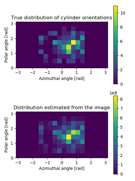
Orientation distributions of cylinders in the image generated in the example. The top panel shows the true distribution, and the bottom panel shows the distribution estimated from the 3D image using the structure tensor method. The distributions show directions corresponding to the whole sphere, but notice that the half-sphere corresponding to the negative \(x\)-values is empty. This happens because the orientations are symmetrical, i.e. directions \(-\vec{r}\) and \(\vec{r}\) describe the same orientation, and therefore half of the possible directions are redundant.
The code used to sample the von Mises-Fisher distribution:
def sample_orientations_from_vonmises_fisher(main_az, main_pol, kappa, n):
        """
        Sample directions from von Mises-Fisher distribution.
        main_az and main_pol give the azimuthal and polar angles of the main direction.
        kappa indicates the spread of the directions around the main direction.
        Large kappa means small spread.
        n gives the number of directions to generate.
        Returns n 3-component unit vectors.

        This code mostly from https://stats.stackexchange.com/questions/156729/sampling-from-von-mises-fisher-distribution-in-python
        but its correctness has not been checked. It seems to
        create plausible results, though.
        """

        import scipy as sc
        import scipy.stats
        import scipy.linalg as la

        def sample_tangent_unit(mu):
                mat = np.matrix(mu)

                if mat.shape[1]>mat.shape[0]:
                        mat = mat.T

                U,_,_ = la.svd(mat)
                nu = np.matrix(np.random.randn(mat.shape[0])).T
                x = np.dot(U[:,1:],nu[1:,:])
                return x/la.norm(x)


        def rW(n, kappa, m):
                dim = m-1
                b = dim / (np.sqrt(4*kappa*kappa + dim*dim) + 2*kappa)
                x = (1-b) / (1+b)
                c = kappa*x + dim*np.log(1-x*x)

                y = []
                for i in range(0,n):
                        done = False
                        while not done:
                                z = sc.stats.beta.rvs(dim/2,dim/2)
                                w = (1 - (1+b)*z) / (1 - (1-b)*z)
                                u = sc.stats.uniform.rvs()
                                if kappa*w + dim*np.log(1-x*w) - c >= np.log(u):
                                        done = True
                        y.append(w)

                return np.array(y)


        def rvMF(n,theta):
                dim = len(theta)
                kappa = np.linalg.norm(theta)
                mu = theta / kappa

                w = rW(n, kappa, dim)

                result = []
                for sample in range(0,n):

                        v = sample_tangent_unit(mu).transpose()
                        v = np.asarray(v.transpose()).squeeze()

                        result.append(np.sqrt(1-w[sample]**2)*v + w[sample]*mu)

                return result


        # First sample directions from the von Mises-Fisher distribution
        main_dir = np.array([np.cos(main_az) * np.sin(main_pol), 1 * np.sin(main_az) * np.sin(main_pol), 1 * np.cos(main_pol)])
        directions = rvMF(n, kappa * main_dir)

        # Convert to orientations (v and -v are the same)
        # by ensuring that all directions have positive x coordinate.
        # This is the same convention used in pi2.
        for dir in directions:
                if dir[0] < 0:
                        dir *= -1

        return directions