Vessel graph
This example demonstrates generation of a vessel graph structure from a tomographic image of vasculature in mouse brain. The analysis process is similar to that used in [1], where it was used to trace vessels in tomographic images of corrosion cast models of cerebral vasculature.
The analysis process consists of thresholding the original image in order to convert it to binary form, where the vessels are white and everything else is black. The binary image is skeletonized into single pixel wide lines, and the lines are traced into a graph structure. Spurious branches are removed using a custom condition based on the ratio of length and diameter of the branch. The average diameter of the branches is calculated and all the information is saved into a .vtk file for further analysis. The figures below represent the same slice through the tomographic image in various processing phases. Also, 3D visualization of the original image and the traced vessels are provided below.
For running this example code, a demonstration image package available at the GitHub releases page is required.
def vessel_tracing():

        # Make binary image where vessels are foreground
        img = pi.read(input_file('orig_basal_ganglia_217'))
        pi.threshold(img, 18000) # The threshold value should be chosen using e.g. Otsu method
        pi.closingfilter(img, 1, True, NeighbourhoodType.BOX) # This closes small holes in the vessels
        pi.convert(img, ImageDataType.UINT8)
        pi.multiply(img, 255)

        # In order to fill cavities in the vessels, fill the background by a temporary color.
        # Here we perform the background fill by a flood fill starting from non-vessel points
        # in the image edge. Here we try to fill from all corners of the image.
        # Note that it is possible that all corners are occupied by vessels and in this case
        # this filling method does not work, but in practice that situation is very rare.
        fill(img, 0, 0, 0)
        fill(img, img.get_width() - 1, 0, 0)
        fill(img, 0, img.get_height() - 1, 0)
        fill(img, img.get_width() - 1, img.get_height() - 1, 0)
        fill(img, 0, 0, img.get_depth() - 1)
        fill(img, img.get_width() - 1, 0, img.get_depth() - 1)
        fill(img, 0, img.get_height() - 1, img.get_depth() - 1)
        fill(img, img.get_width() - 1, img.get_height() - 1, img.get_depth() - 1)
        # Here the vessels, cavities and background have colors 255, 0, and 128, respectively.
        # Set cavities and vessels to 255 and background to 0.
        pi.replace(img, 255, 0)
        pi.replace(img, 0, 255)
        pi.replace(img, 128, 0)

        pi.writeraw(img, output_file('vessel_bin'))

        # Now calculate skeleton. We use the surfaceskeleton function and specify False as second
        # argument to indicate that we want a line skeleton. In many cases this method makes
        # more stable skeletons than the lineskeleton function.
        pi.surfaceskeleton(img, False)
        pi.writeraw(img, output_file('vessel_skele'))

        # Below we will need the distance map of vessel phase, so we calculate it here.
        img = pi.read(output_file('vessel_bin'))
        dmap = pi.newimage(ImageDataType.FLOAT32)
        pi.dmap(img, dmap)
        pi.writeraw(dmap, output_file('vessel_dmap'))
        dmap_data = dmap.get_data()


        # Trace skeleton
        skeleton = pi.read(output_file('vessel_skele'))
        smoothing_sigma = 2
        max_displacement = 2
        vertices = pi.newimage(ImageDataType.FLOAT32)
        edges = pi.newimage(ImageDataType.UINT64)
        measurements = pi.newimage(ImageDataType.FLOAT32)
        points = pi.newimage(ImageDataType.INT32)
        pi.tracelineskeleton(skeleton, vertices, edges, measurements, points, True, 1, smoothing_sigma, max_displacement)


        # Next, we will remove all edges that has at least one free and and whose
        # L/r < 2.
        # First, get edges, vertices, and branch length as NumPy arrays.
        old_edges = edges.get_data()
        vert_coords = vertices.get_data()

        # The tracelineskeleton measures branch length by anchored convolution and returns it in the
        # measurements image.
        meas_data = measurements.get_data()
        length_data = meas_data[:, 1]


        # Calculate degree of each vertex
        deg = {}
        for i in range(0, vert_coords.shape[0]):
                deg[i] = 0

        for i in range(0, old_edges.shape[0]):
                deg[old_edges[i, 0]] += 1
                deg[old_edges[i, 1]] += 1

        # Determine which edges should be removed
        remove_flags = []
        for i in range(0, old_edges.shape[0]):
                n1 = old_edges[i, 0]
                n2 = old_edges[i, 1]

                # Remove edge if it has at least one free end point, and if L/r < 2, where
                # r = max(r_1, r_2) and r_1 and r_2 are radii at the end points or the edge.
                should_remove = False
                if deg[n1] == 1 or deg[n2] == 1:

                        p1 = vert_coords[n1, :]
                        p2 = vert_coords[n2, :]

                        r1 = dmap_data[int(p1[1]), int(p1[0]), int(p1[2])]
                        r2 = dmap_data[int(p2[1]), int(p2[0]), int(p2[2])]

                        r = max(r1, r2)
                        L = length_data[i]

                        if L < 2 * r:
                                should_remove = True

                # Remove very short isolated branches, too.
                if deg[n1] == 1 and deg[n2] == 1:
                        L = length_data[i]
                        if L < 5 / 0.75: # (5 um) / (0.75 um/pixel)
                                should_remove = True

                remove_flags.append(should_remove)

        remove_flags = np.array(remove_flags).astype(np.uint8)
        print(f"Before dynamic pruning: {old_edges.shape[0]} edges")
        print(f"Removing {np.sum(remove_flags)} edges")

        # This call adjusts the vertices, edges, and measurements images such that
        # the edges for which remove_flags entry is True are removed from the graph.
        pi.removeedges(vertices, edges, measurements, points, remove_flags, True, True)


        # Convert to vtk format in order to get radius for each point and line
        vtkpoints = pi.newimage()
        vtklines = pi.newimage()
        pi.getpointsandlines(vertices, edges, measurements, points, vtkpoints, vtklines)

        # Get radius for each point
        points_data = vtkpoints.get_data()
        radius_points = np.zeros([points_data.shape[0]])
        for i in range(0, points_data.shape[0]):
                p = points_data[i, :]
                r = dmap_data[int(p[1]), int(p[0]), int(p[2])]
                radius_points[i] = r


        # Get average radius for each branch
        # Notice that the vtklines image has a special format that is detailed in
        # the documentation of getpointsandlines function.
        lines_data = vtklines.get_data()
        radius_lines = []
        i = 0
        edge_count = lines_data[i]
        i += 1
        for k in range(0, edge_count):
                count = lines_data[i]
                i += 1

                R = 0
                for n in range(0, count):
                        index = lines_data[i]
                        i += 1
                        p = points_data[index, :]
                        R += dmap_data[int(p[1]), int(p[0]), int(p[2])]
                R /= count

                radius_lines.append(R)

        radius_lines = np.array(radius_lines)


        # Convert to vtk format again, now with smoothing the point coordinates to get non-jagged branches.
        vtkpoints = pi.newimage()
        vtklines = pi.newimage()
        pi.getpointsandlines(vertices, edges, measurements, points, vtkpoints, vtklines, smoothing_sigma, max_displacement)


        # Write to file
        pi.writevtk(vtkpoints, vtklines, output_file('vessels'), "radius", radius_points, "radius", radius_lines)
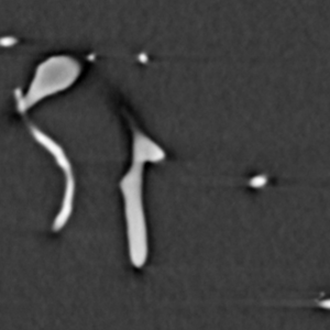
Input image. The bright regions are corrosion-cast blood vessels.

Segmented vessels.
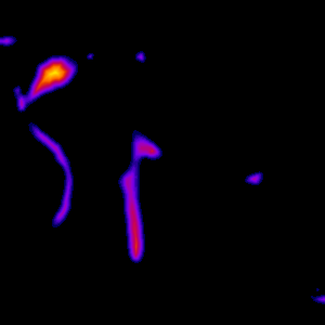
Distance map of the segmented vessels.

Skeleton of the segmented vessels.
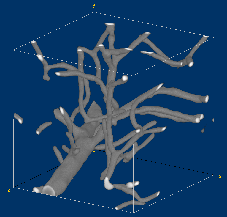
Volume visualization of the original vessel image. This visualization has been generated with the Volume Viewer plugin of Fiji.
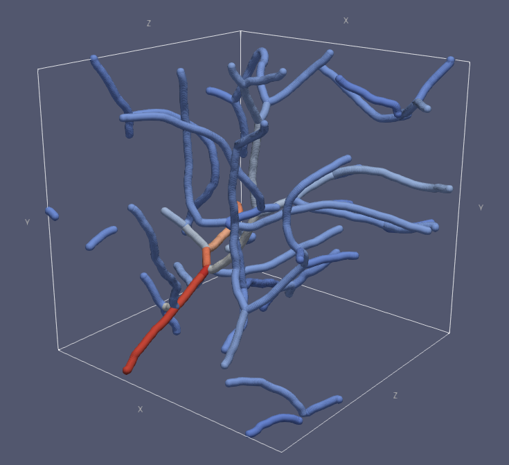
Visualization of the traced vessels. Each vessel branch has been colored based on the average diameter of that branch. Bright colors correspond to large diameters. This visualization has been generated with ParaView.
References
[1] Wälchli T., Bisschop J., Miettinen A. et al. Hierarchical imaging and computational analysis of three-dimensional vascular network architecture in the entire postnatal and adult mouse brain. Nature Protocols, 2021.