Finding surface using Edwards-Wilkinson model

This example shows how to find a surface or interface from a grayscale image.

Surface recognition is done using the ‘Carpet’ algorithm according to Turpeinen - Interface Detection Using a Quenched-Noise Version of the Edwards-Wilkinson Equation. The algorithm places a surface at \(z=0\), and moves it towards larger \(z\) values according to the Edwards-Wilkinson equation. The movement of the surface stops when it encounters enough pixels with value above specific stopping gray level. The surface does not move through small holes in the object as it has controllable amount of surface tension. The output of the algorithm is a height map that gives the \(z\)-position of the surface for each \((x, y)\)-location. In addition to the height map, a visualization of the evolution of the surface can be made.

After finding the surface, the example demonstrates how to visualize it.

Visualization of the evolution of an Edwards-Wilkinson surface on top of the original data. The figure shows one \(xz\)-slice through the original image. The surface has been drawn with red. The animation shows the surface as a function of iteration (i.e. time).

def find_surface():
        """
        Demonstrates surface recognition using Edwards-Wilkinson model.
        """

        # Read image
        orig = pi.read(input_file())

        # Crop smaller piece so that the surface does not 'fall through'
        # as there's nothing in the edges of the image.
        # Usually surfaces are recognized from e.g. images of paper sheet
        # where the sheet spans the whole image.
        img = pi.newimage(orig.get_data_type())
        pi.crop(orig, img, [80, 90, 0], [85, 120, orig.get_depth()])

        pi.writeraw(img, output_file('findsurface_geometry'))

        # This image will hold the height map of the surface
        hmap = pi.newimage(ImageDataType.FLOAT32)

        # ... and this one will be a visualization of surface evolution
        vis = pi.newimage(orig.get_data_type())

        # Now find the surface.
        # We will stop at gray level 100 and perform 60 iterations
        # with surface tension 1.0.
        pi.findsurface(img, hmap, 100, Direction.DOWN, 1.0, 60, 1, vis, img.height() / 2, 900)

        # Save the result surface
        pi.writeraw(hmap, output_file('findsurface_height_map'))

        # Save the visualization
        pi.writeraw(vis, output_file('findsurface_evolution'))



        # We can also draw the surface to the image
        surf_vis = pi.newimage()
        pi.set(surf_vis, img)
        pi.drawheightmap(surf_vis, hmap, 900)
        pi.writeraw(surf_vis, output_file('findsurface_full_vis'))

        # Or set pixels below or above the surface.
        # This is useful to, e.g., get rid of background noise above
        # or below the surface of the sample.
        before_vis = pi.newimage()
        pi.set(before_vis, img)
        pi.setbeforeheightmap(before_vis, hmap, 900)
        pi.writeraw(before_vis, output_file('findsurface_before_vis'))

        after_vis = pi.newimage()
        pi.set(after_vis, img)
        pi.setafterheightmap(after_vis, hmap, 900)
        pi.writeraw(after_vis, output_file('findsurface_after_vis'))

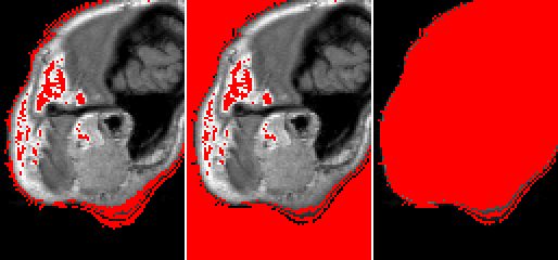
Visualizations of the found surface (red) at single \(xy\)-slice of the input (grayscale). The left panel shows the surface, the middle panel shows all the pixels that are located above the surface and the right panel all the pixels that are below it.